Continuous Variation: Skills (SL IB Biology)

Variation can be discrete or continuous

• Discrete variation is variation that falls into two or more clear-cut categories with no overlap or in-between categories
  • Blood group is an example of discrete variation
  • All human blood is either group O, A, B or AB, each with a Rhesus factor (+ or -)
• This gives just 8 distinct blood groups:

Pie chart showing global blood group distribution

Worldwide A, B, O blood group distribution by percentage, 2019

(data varies regionally with ethnicity)

Continuous Variation

• Continuous variation occurs when two or more genes affect the final characteristic
• For example, height in humans is determined by many genetic factors:
  • Bone length
  • Skeletal muscle structure
  • Ability to absorb food substances effectively
  • Hormone production
  • …As well as environmental factors like diet, exercise, prenatal nutrition, lifestyle etc
• Most characteristics are determined by more than one gene - a polygenic characteristic
• Even grouped data like shoe size appears to be discrete but in fact, peoples' feet vary continuously in size
  • Shoe size is merely a practicality for shoe manufacturers, who cannot make exactly the right-sized shoes for everybody
• Continuous variation in birth mass results in the population displaying a normal distribution (bell-shaped curve)
  • Environmental factors can also affect birth mass, e.g. mother's diet, presence of a twin, smoking etc
• Continuous variation occurs when there are quantitative differences in the phenotypes of individuals within a population for particular characteristics
• Quantitative differences do not fall into discrete categories like in discontinuous variation
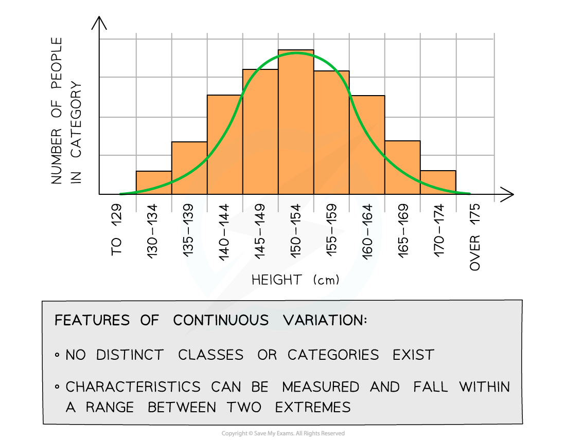
  • For example, the mass or height of a human is an example of continuous variation
  • Instead for these features, a range of values exist between two extremes within which the phenotype will fall
• The lack of categories and the presence of a range of values can be used to identify continuous variation when it is presented in a table or graph

Normal distribution curve

Graph showing population variation in height: an example of continuous variation with quantitative differences

Genetic basis of continuous variation

• This type of variation is caused by an interaction between genetics and the environment
• Phenotype = genotype + environment
• At the genetic level:
  • Different alleles at a single locus have a small effect on the phenotype
  • Different genes can have the same effect on the phenotype and these add together to have an additive effect
  • If a large number of genes have a combined effect on the phenotype they are known as polygenes
• An example of a continuous polygenic trait is skin colour
• Skin colour is determined by several genes that cause the production of a protein called melanin
  • The more melanin is produced, the darker the skin pigmentation becomes
• Skin colour is also influenced by environmental factors such as UV exposure, which can cause the skin colour to become darker

Comparison of Continuous and Discontinuous Variation Table

What are box plots and when should they be used?

• Box plots are also known as box-and-whisker diagrams
• They are used when we are interested in splitting data up into quartiles
• Using quartiles and drawing a box plot allows us to see what is happening at the low, middle and high points and consider any possible extreme values

How to draw a box plot

• You need to know five values to draw a box plot
  • Lowest data value
  • First quartile
  • Median
  • Third quartile
  • Highest data value
• Usually on graph paper, box plots are drawn accurately with the five points marked by short vertical lines
  • The middle three values then form a box with the median line inside
    • The median will not necessarily be in the middle of the box
  • The box represents the interquartile range (middle 50% of the data)
  • The lowest data value and highest data value are joined to the box by horizontal lines
    • These are often called whiskers
    • They represent the lowest 25% of the data and the highest 25% of the data
• You may be given a box plot
  • From which you can read off the five values
  • Calculate other statistics like the range and interquartile range (IQR)

Outliers

• Outliers are data points that exist at the extremes above and below the rest of the data
• In order for a data point to be categorised as an outlier it needs to be more than 1.5 × the interquartile range above the third quartile or below the first quartile
• As shown in the worked example above, the outliers are plotted separately to the whiskers of the plot